Homework

HW1 – Free Fall
Write a program that calculates the time it takes for a ball to drop from a user specified height to reach the ground. Use argparse. Also the user to choose different values of gravity. And any other features you think maybe interesting.

HW2 – Exercise 5.3: Integration
Consider the integral

$E(x) = \int^x_0 e^{-t^2} dt$

a) Write a program to calculate E(x) for values of x from 0 to 3 in steps of 0.1. Choose for yourself what method you will use for performing the integral and a suitable number of slices.
b) When you are convinced your program is working, extend it further to make a graph of E(x) as a function of x.
Note that there is no known way to perform this particular integral analytically, so numerical approaches are the only way forward.

HW3 – Exercise 6.16: The Lagrange Point
There is a magical point between the Earth and the Moon, called the L₁ Lagrange point, at which a satellite will orbit the Earth in perfect synchrony with the Moon, staying always in between the two. This works because the inward pull of the Earth and the outward pull of the Moon combine to create exactly the needed centripetal force that keeps the satellite in its orbit. Here’s the setup:

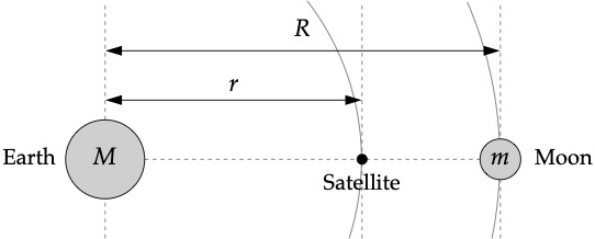
Assuming circular orbits, and assuming that the Earth is much more massive than either the Moon or the satellite, show that the distance r from the center of the Earth to the L₁ point satisfies

${GM\over r^2} - {Gm\over(R-r)^2} = \omega^2 r,$

where M and m are the Earth and Moon masses, G is Newton’s gravitational constant, and ω is the angular velocity of both the Moon and the satellite.
The equation above is a fifth-order polynomial equation in r (also called a quintic equation). Such equations cannot be solved exactly in closed form, but it’s straightforward to solve them numerically. Write a program that uses either Newton’s method or the secant method to solve for the distance r from the Earth to the L₁ point. Compute a solution accurate to at least four significant figures.
The values G and the Earth’s mass can be found in the astropy.constants or scipy.constants sub-packages. The Moon’s mass is 7.348e22 kg and the Eart-Moon distance is 3.844e8 m. The value of ω is 2.662e-6 s^-1. You will also need to choose a suitable starting value for r, or two starting values if you use the secant method.

HW4 – Fourier Analysis – Time Series Analysis
Many astrophysical phenomena very over short enough time scales that they can be observed by humans. One of the strongest time varying signals are occulting binaries, when two orbiting stars pass in front of one-another. This website has data from the TESS machine that observed hundreds of nearby stars. You can download the data for a light curve as a fits file from the site after you choose a star. You can read the file using astropy

from astropy.io import fits
hdul = fits.open(filename)
times = hdul[1].data['times']
fluxes = hdul[1].data['fluxes']
ferrs = hdul[1].data['ferrs']

Note that these files contain errors on the measured fluxes that we will not use in Fourier analysis. If you plot a light curve you’ll see that these observations have lots of points and then a long time and then lots of points. This is how the observations were done, with the telescope on the object for some set amount of time and then revisiting the object many months or years later. Choose an epoch with lots of observations and reduce your data to just that range. Create the Fourier transform for that range and plot the power spectrum. See how few coefficients you can use to capture the behavior of the eclipsing binary looking at the inverse transform. You can check a different region of the light curve and redo the analysis to see if you get the same results.

An extra complication. The TESS data is almost evenly spaced. The observations were done evenly spaced, but there will be some missing data because things happen. If you look at the times in the file, you can identify the missing time steps. You can try filling this in with linear interpolation and then redoing the Fourier analysis. Because the TESS data is so good, this won’t make much of a difference. If the light curve was much more unevenly sampled the Fourier transform would be totally wrong. This is how most astronomy data is and dealing with those problems is what much of time series analysis is about.

HW5 – Monte Carlo Radiative Transfer
One of the most common uses of Monte Carlo calculations in astrophysics is for radiative transfer. The simplest example of this is the motion of radiation in a star. The cores of stars are hot and dense, such that all electrons are ionized and the cross section for most photons to interact with an electron is just the frequency independent Thompson cross-section.

$\sigma_T = \frac{8\pi}{3} \big(\frac{e^2}{4\pi \epsilon_0 m_e c^2}\big)^2 = 6.652 \times10^{-25} cm^2$

Another import quantity to consider in scattering theory is the mean free path of a particle.

$l = 1/(n \times\sigma)$

If $n_e = 10^{20} cm^{-3}$ the mean free path would be 150m. Start by just considering a slab of constant electron density with this value and a width of 1km. Perform a Monte Carlo simulation of a photon through this slab. Note that for low energy photons ( $E = hf << m_e c^2$ ) the photon scattering is isotropic, equally likely in any direction. However, since you are only trying to follow the photons progress through the slab, you only need to consider the angle the scattered photon makes with the direction through the slab. Also note that your photon is almost as likely to be reflected back to the beginning as make it through the slab, so make sure you account for this possibility. Make an animation of your photons path. One example of how to make an animation can be found here.

Now to extend this calculation to the Sun we need to know the Sun’s electron density as a function of radius. A reasonably accurate fit is given as equation 4.2 in Neutrino Astrophysics by John Bachall. The formula is

$n_e(r) = 2.5 \times 10^{26} exp^{-\frac{r}{0.096 R_{sun}}} cm^{-3}$

where $R_{sun}$ is the solar radius, 696,340km. The formula is only good to $0.9R_{sun}$ , after which density drops quickly and one can assume there are no more scatterings for photons. We can now calculate the time it takes for a photon to escape the Sun. Note that the mean free path changes by many orders of magnitude as the radius changes. So you can’t simply ask what is the probability of a photon scattering for some fixed distance, like 1cm. Instead, just like for radioactive decay, we can draw how far the photon traveled before a scattering from the exponential distribution.

$P(x) = \frac{1}{l} e^{-x/l}$

So to simulate the photons path, start at r=0, calculate the electron density and from that the mean free path. Draw a random number from the exponential distribution with a scale of the mean free path. And update r. Calculate the new electron density, the new mean free path and the angle the photon was scatter by (just 0 to 180 because we only care about relative to r) and then draw a new random number from the exponential distribution with the new mean free path. Note you must keep track of both r, the distance from the Sun’s center and s, the total distance traveled by the photon, as the total distance is the time, t = cs.

HW6 – Exercise 8.8: Space Garbage

A heavy steel rod and a spherical ball-bearing, discarded by a passing spaceship, are floating in zero gravity and the ball bearing is orbiting around the rod under the effect of its gravitational pull.

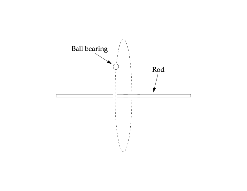
For simplicity we will assume that the rod is of negligible cross-section and heavy enough that it doesn’t move significantly, and that the ball bearing is orbiting around the rod’s mid-point in a plane perpendicular to the rod.

a) Treating the rod as a line of mass M and length L and the ball bearing as a point of mass m, convince yourself that the attractive force F felt by the ball bearing in the direction toward the center of the rod is give by of

$F = \frac{GMm}{\sqrt{(x^2 + y^2)(x^2 + y^2 + \frac{1}{4}L^2)}}$

Hence one finds that the equations of motion for the position (x,y) of the ball bearing in the xy-plane are

$\frac{d^2 x}{dt^2} = -GM \frac{x}{r^2\sqrt{r^2 + \frac{1}{4}L^2}} \, \, \, \frac{d^2 y}{dt^2} = -GM \frac{y}{r^2\sqrt{r^2 + \frac{1}{4}L^2}}$

where $r = \sqrt{x^2 + y^2}$ .

b) Convert these two second-order equations into four first-order equations. Then working in units of G = 1, write a program to solve for M=10, L=2 and initial conditions (x,y) = (1,0) with a velocity of +1 in the y direction. Calculate the orbit from t=0 to t=10 and make a plot of it, meaning a plot of y against x. You should find that the ball bearing does not orbit in a circle or an ellipse as a planet does, but has a precessing orbit, which arises because the attractive force is not 1/r² as it is for the Sun.

This entry is licensed under a Creative Commons Attribution-NonCommercial-ShareAlike 4.0 International license.

Computational Methods

Course on computational methods used in physics

Need help with the Commons?